Image Generation Guide
The goal of this guide is to help the curious reader understand the technical foundations, applications, and challenges of image generation. We cover the key ideas and link to high-quality reference material for further learning.
- What is image generation?
- What are diffusion models?
- Challenges
- Technical Foundations
- Glossary
- Recommended References
What is image generation?
Image generation refers to the process of creating images using pre-trained models.
You've likely seen AI-generated images and videos online. Maybe you've generated your own images using applications like DALL-E or MidJourney. This guide can help you dive deeper.
Image generation is a wide and active area of research. This guide focuses on a subset of essential topics:
- Forward and reverse diffusion, the processes that enables today's popular diffusion models to generates images,
- Stable Diffusion, a flexible, open-source diffusion model architecture, and
- Challenges in achieving a desired visual style and meeting performance requirements (e.g. speed, memory).
This guide does not attempt cover all topics. We omit or gloss over:
- Alternative neural network architectures for image generation like
GANs - Training details like hyperparameters, loss functions, and benchmarks
- Environment setup, getting started, and hardware considerations
- Neural Network fundamentals (e.g. stochastic gradient descent)
What are diffusion models?
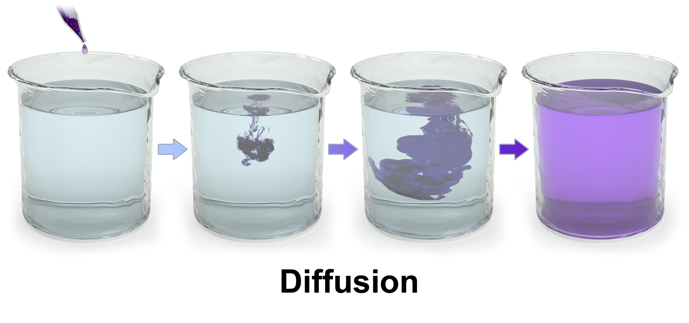
Diffusion comes from the latin diffundere, meaning "to spread out". It is the familiar process of things moving from higher concentration to lower concentration.
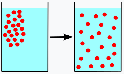
When purple dye is dropped into water, the dye diffuses until the entire mixture has a uniform purple hue. That is, until distribution of molecules from the purple dye is uniformly random.
Diffusion models are based on an analogous process.
First, we collect images that look like what we want our model to generate. Each image is like a drop of "purple dye", rich in information and decidedly non-random.
Next, we add increasing levels of noise to each image. We continue this diffusion process until the information has been "systematically destroyed". (That is, until the image has become uniform random noise.)
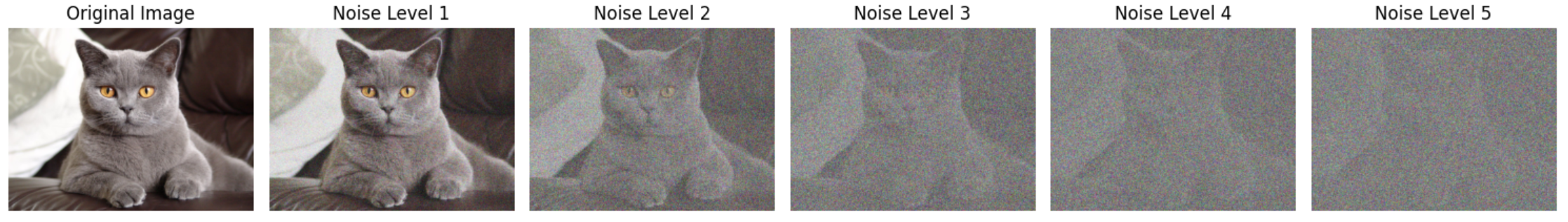
Noisy images are paired with their originals to form a training data set. We use this data set to train a model to recover the original image given a noisy image. In other words, the model attempts to remove the noise we added.
The model's loss function measures the difference between generated output and the original images, allowing us to improve the model parameters the usual way (stochastic gradient descent).
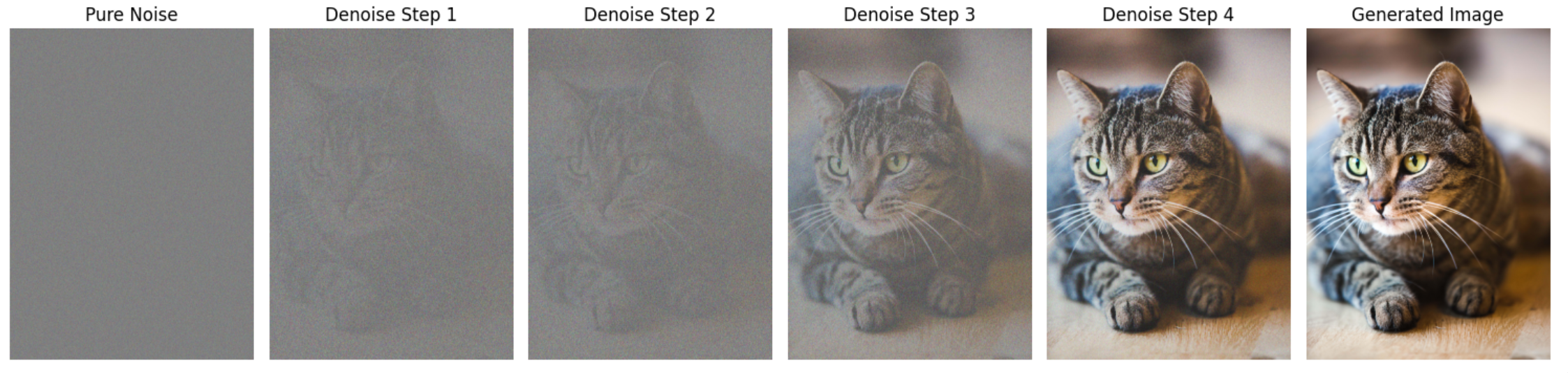
After training the model, we can use it to generate new images: If we start with pure noise, the model will "denoise" it into something that looks like it could be from the training set's original images.
We'll discuss diffusion models in more detail in the Technical Foundations section. First, let's consider some of the challenges we encounter when working with diffusion models.
Challenges
Selecting a base model
If you are like most developers, you will not need to train diffusion models from scratch. Instead, you will select a pre-trained base model and either use it for inference directly or fine-tune it to your needs. (We'll mention several viable methods of fine-tuning in a later section.)
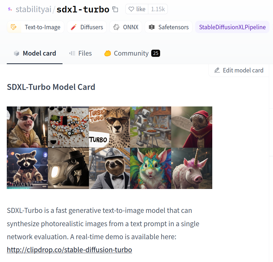
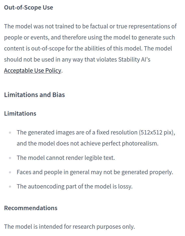
Like any AI model, generative image models reflect biases in their training data. It is important to choose models whose training data, terms of use, and degree of openness are consistent with your values and needs.
Hugging Face hosts a large collection of models available for free download. Each model has a model card that describes its origin, capabilities, limitations and terms of use.
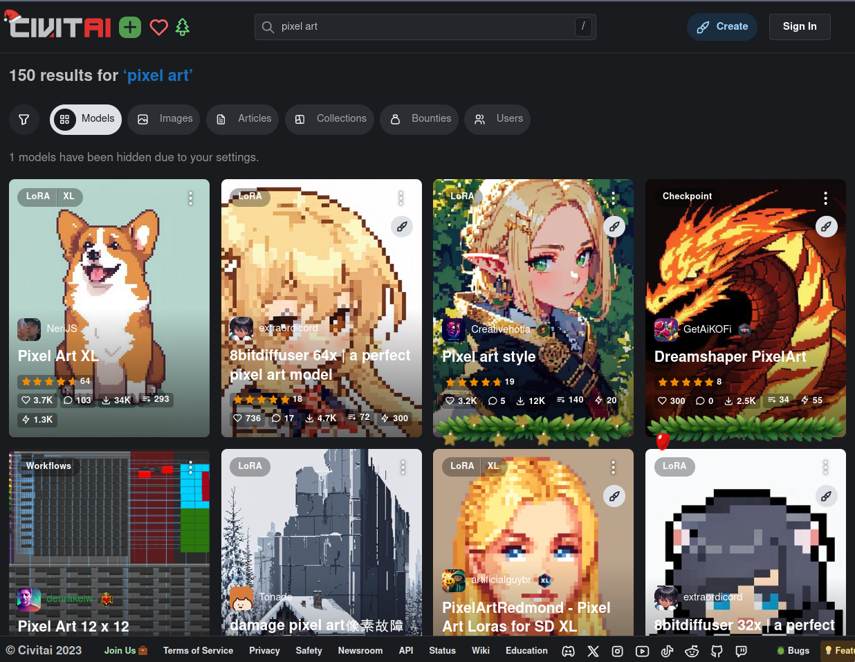
Civit AI offers a search tool for finding models that are already fine-tuned to produce a specific style.
Conditioning and Control
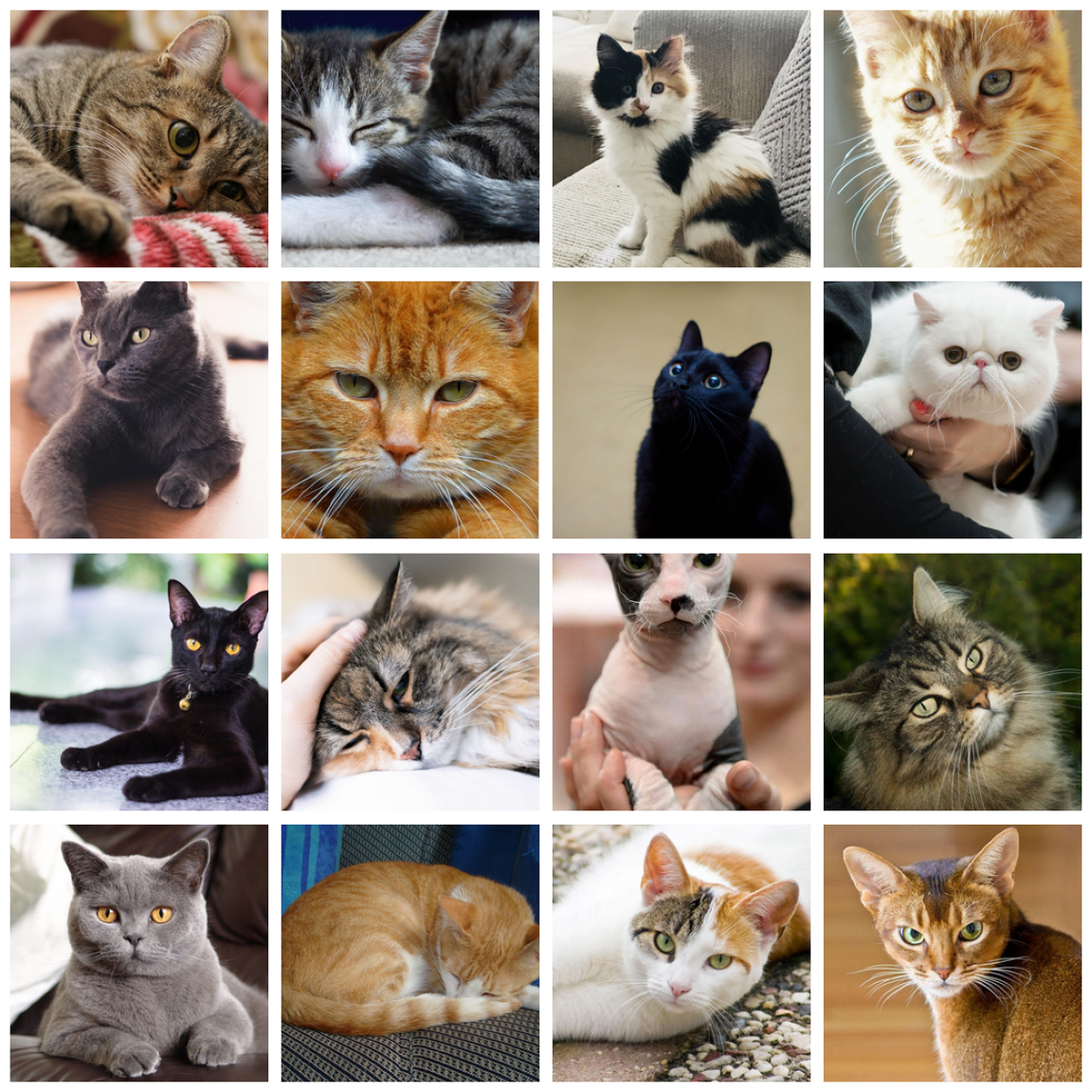
The most basic form of image generation is called unconditional image generation. Unconditional image generation means producing images that look like a random sample of the model's training data, with no additional input. If our training set contains pictures of cats, our model will generate pictures of cats. If our training set contains pictures of boats, our model will generate pictures of boats.
The real power of diffusion models comes from our ability to condition on various types of input data in order to tailor the output to our specific needs. When models make use of multiple types of data, we call them multi-modal. We'll consider a few examples.
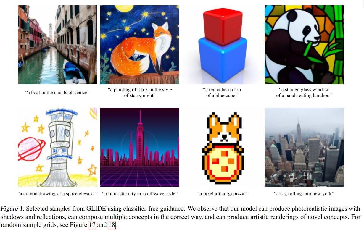
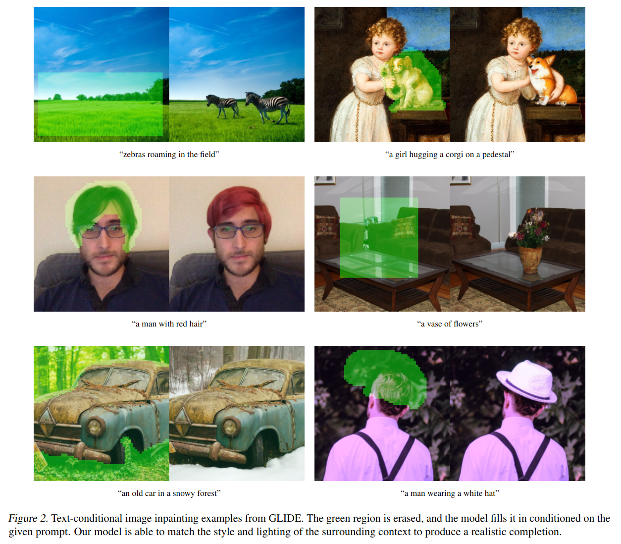
CLIP and GLIDE allow models to be conditioned by text, enabling tasks like Text-to-Image and Inpainting.
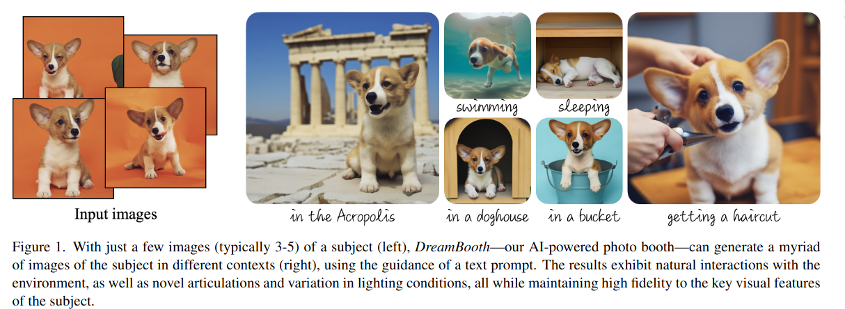
Fine-tuning and transfer learning via techniques like Dreambooth and Textual Inversion allow a model to produce outputs of a specific subject or art style.
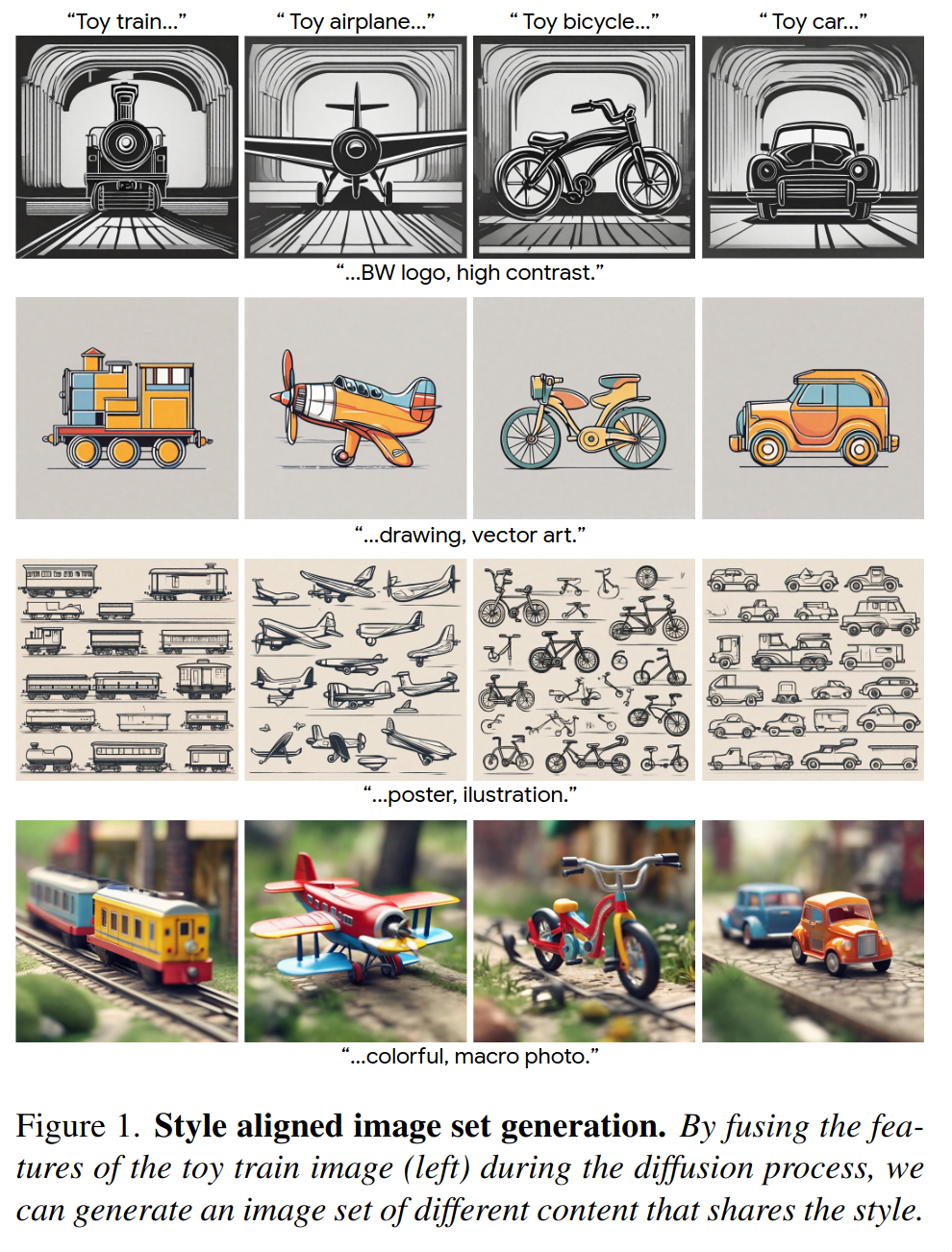
In some cases, style-transfer can even be achieved without fine-tuning, as shown by Style Aligned
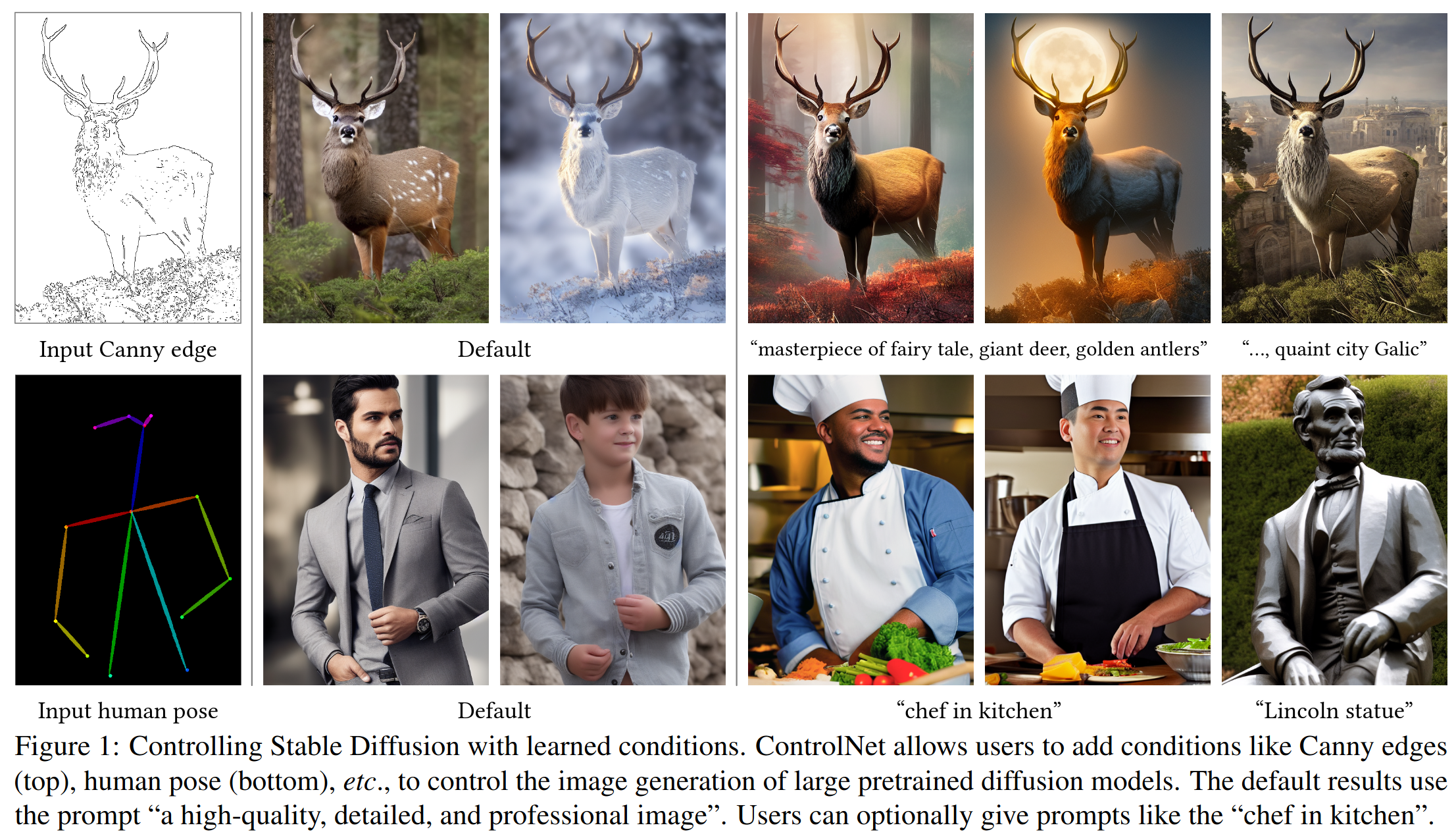
Control Nets are complementary models that, once trained, allow the output of a diffusion model to be conditioned on (i.e. controlled by) skeletal animation poses, depth maps, segmentation maps, canny edges, and more. Control Nets showed how to go beyond text conditioning and opened up a huge number of previously infeasible use-cases for image generation.
Consistency for video
We use Control Nets and style transfer so that we can generate images with consistent style and form, but the challenge of consistency goes beyond these techniques. Image-to-video models must additionally achieving consistency across video frames.
At the time of this writing, models are still in the early days of being trained to understand and generate video, with companies like RunwayML exploring what they're calling General World Models.
Performance
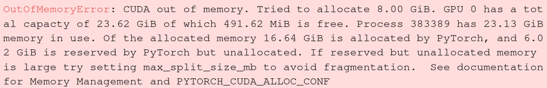
Image generation requires significant compute and memory resources. Since entire models are typically loaded into GPU memory, you will need to consider the capabilities and limitations of the systems on which your models run, so as to not exceed them.
Depending on the use case, it may be best prioritize inference speed over image quality, or vice versa.
If a model is too large to fit into GPU memory, quantization allows us to lower the memory requirements: If a model made up of 32-bit floats is too large, you can convert all the 32-bit floats to 16-bit floats, 8-bit floats, or even 4-bit floats. Downsizing floats reduces precision, but may allow models to run on less powerful hardware. Quantization of float32 models to float16 reduces memory requirements considerably without appreciable reduction in image quality.
Tom ("TheBloke") Jobbins has released over 3000 models on Hugging Face. He uploads variants of popular models: quantized, fine-tuned, and with different file formats. He helps developers onboard into AI and run models on a wide variety of hardware. In August 2023, a16z awarded Tom a grant for his contributions to open source.
Performance considerations affect everything from training, inference, and offering cloud services to end users. Here are a few references from Hugging Face:
- The accelerate python package simplifies running PyTorch code across multiple devices (a "distributed configuration").
- These jupyter notebooks discuss some techniques / considerations for speeding up inference of diffusion models: Accelerate inference, Effective and efficient diffusion
- This section of the
diffusersdocs considers many aspects of optimization: Optimization Overview
Technical Foundations
There are many ways to generate images, which can make it difficult to learn the technical details. It helps to learn a specific example end-to-end, rather than trying to learn abstract general principles.
We will focus on Stable Diffusion, a popular, open-source, and extensible model for image generation. We will also cover Control Nets, the flexible way of adding various conditioning to a stable diffusion model's outputs.
Prerequisites
Before diving into the details of Stable Diffusion, we recommend familiarizing yourself with the following topics, which this guide will not cover:
| Term | Description |
|---|---|
| Tensors | Multidimensional arrays of numbers, used as the basic data structure in neural networks to represent inputs, outputs, weights, etc. |
| Inputs | Tensors fed into a neural network model. They represent the data the model will process. |
| Outputs | The results produced by a neural network model when given an input. |
| Loss | A measure used during training to quantify how far a model's outputs are from the desired output. It guides the updating of the model's parameters. |
| Parameters | The internal variables of a model that are adjusted during training to minimize loss. These include weights and biases in the network. |
| Layers/Blocks | Organizational units of parameters within a neural network. Layers are composed of neurons and perform specific functions, while blocks are groups of layers working together. |
| Training | The phase in which a neural network learns from data to create a foundational model. It involves adjusting parameters to minimize loss. |
| Inference | The phase where a trained neural network model is used to make predictions or generate outputs based on new inputs. |
| Fine-tuning | An optional training phase that adjusts a pre-trained model to specific tasks or datasets, refining its performance. |
| Model Architectures | The specific configuration of layers, blocks, or neural networks within a larger system, defining the structure and behavior of the model. |
Stable Diffusion and Control Nets
Stable Diffusion and Control Net have several components that work together to generate images. Architecture diagrams found in these systems' research papers assume the reader already understands the basic components involved. For example, consider the following diagrams from the Stable Diffusion and Control Net papers, respectively.
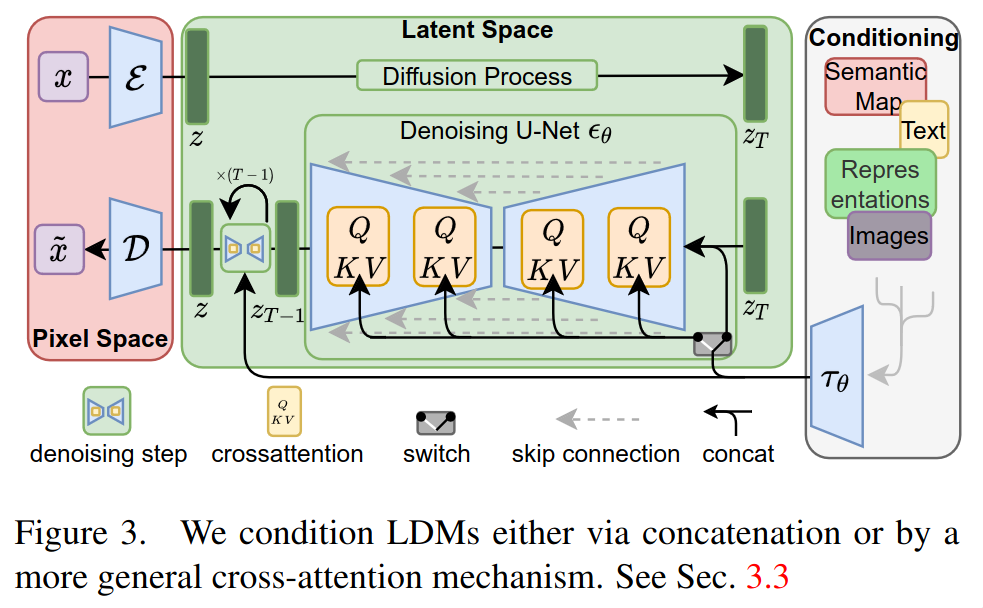
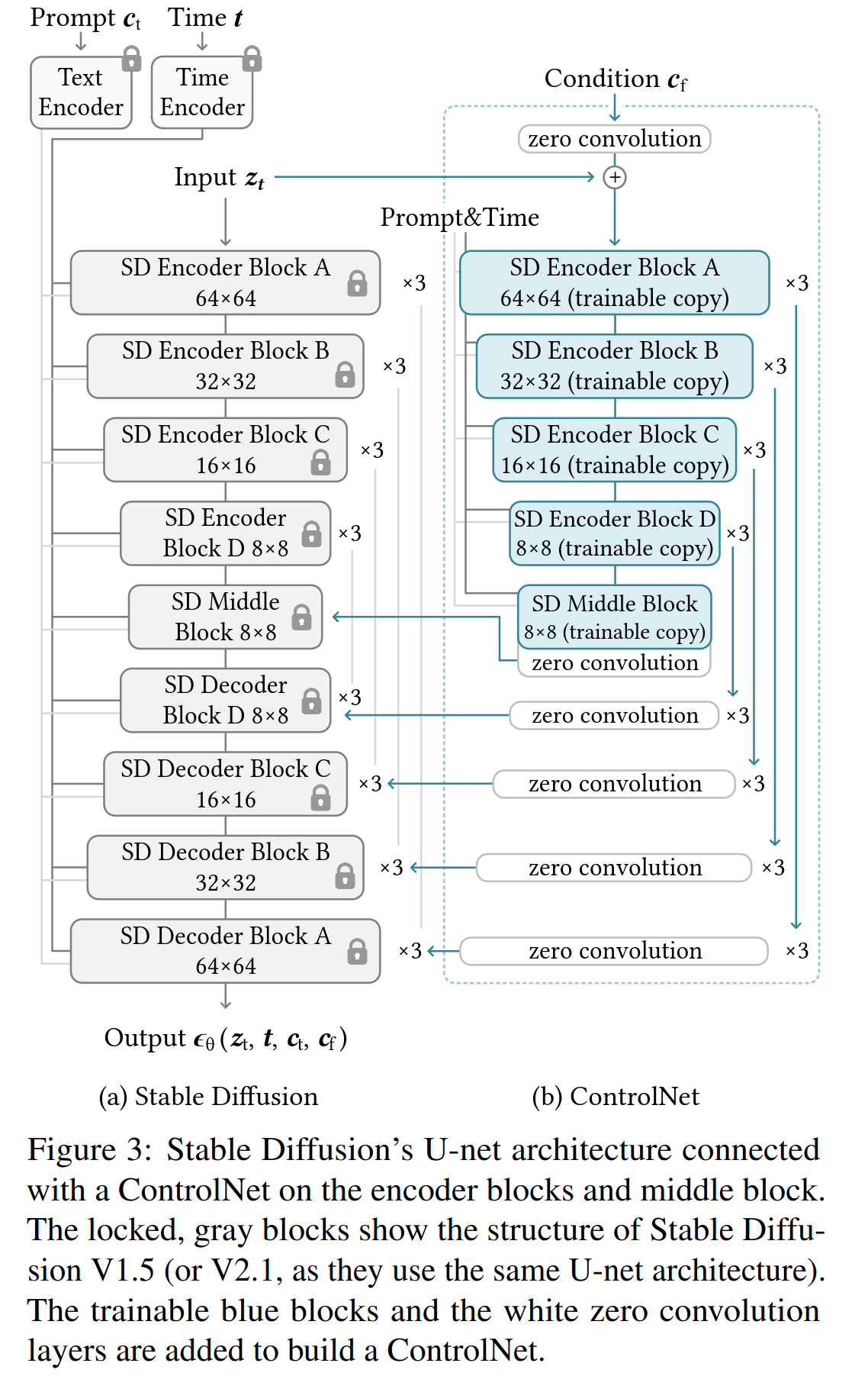
By the end of this guide article, we hope you are able to understand these diagrams (and the text) from the original research papers.
We will start with a diagram showing the entire architecture at a high level. Then we will examine the individual components until we know each component does and how it is trained.
As you read, you may refer to the glossary for definitions of key terms and the recommended references for more complete explanations. It will likely help to read through the glossary at least once before continuing.
The entire pipeline
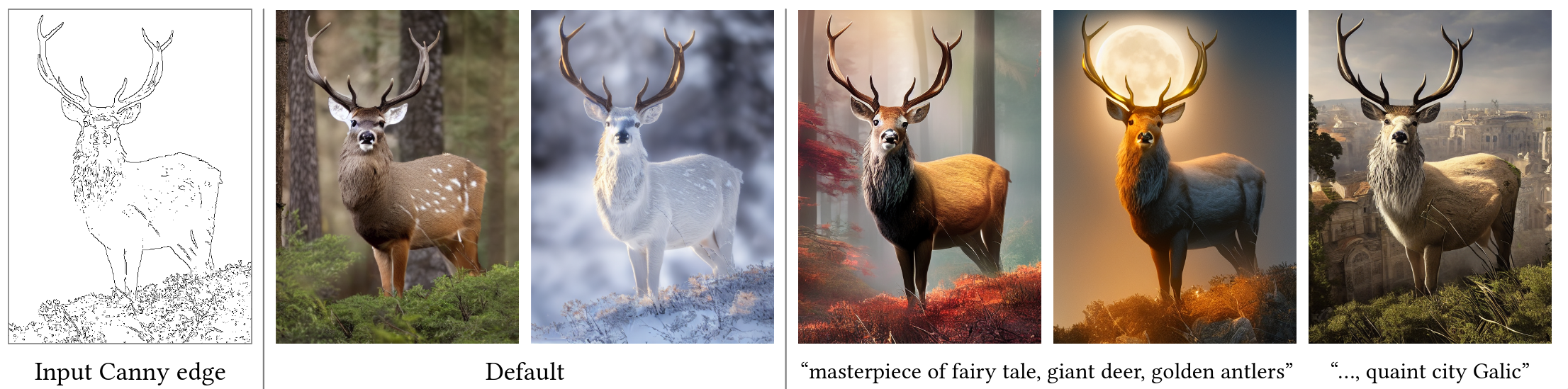
Let's examine the entire Stable Diffusion pipeline, including text conditioning and a Control Net trained on Canny edge maps.
The following diagram illustrates the data flow in Stable Diffusion with a Control Net. Refer to the glossary and followup sections for more details about each component.

Inputs and Outputs
- Input: Text input and conditional input (Canny edge map).
- Output: Final generated image post reverse diffusion.
Process Overview
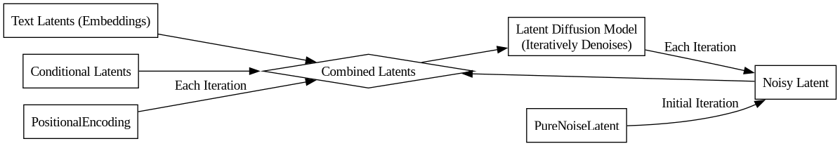
- Noisy Latent Initiation: The process begins with a latent generated from pure noise.
- Text and Conditional Inputs Processing: Text input and a Canny edge map are processed by their respective encoders to produce latent representations.
- Combining Latents: The noise latent, text latent, image latent, and positional encoding (indicating the initial timestep) are combined into a comprehensive "noisy latent". This combination serves as a comprehensive input to the U-Net.
- U-Net Encoding and Decoding: The combined latents pass through the U-Net encoder, which includes Control Net's trainable copy. The encoder's residual connections and Control Net's zero convolutions feed into the U-Net decoder, which predicts the latent noise, conditioned on the various inputs.
- Iterative Reverse Diffusion: A scheduler adjusts the predicted noise - subtracting a portion of it and adding new noise to the latent. The updated noisy latent, now recombined, re-enters the U-Net for further processing. This loop continues, incrementing the timestep and updating positional encoding each iteration, until a predefined number of steps is reached.
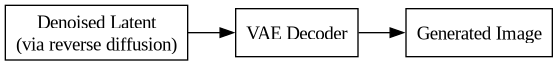
- Final Image Generation with VAE Decoder: The process ends with the VAE decoder transforming the denoised latent into the final image. Notice that the VAE encoder is not required for this (noise-to-image) task, though it was needed during training and would be needed for image-to-image tasks.
In the following sections, we'll inspect the Stable Diffusion pipeline in more detail, providing simple diagrams and brief explanations of each component.
The recommended resources contains more complete explanations of each component.
Diffusion Model
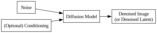
Input: Randomly generated noise (optionally combined with non-random "conditioning" inputs like text, canny edge maps, etc).
Output: A coherent generated image, produced from several iterative reverse diffusion steps.
Training: The training process for a diffusion model involves learning to denoise images. Once the model can reconstruct original images from noisy inputs, we use it to generate new images from (pure or conditioned) noise.
Clarification: The term "diffusion model" does not refer to a specific architecture or arrangement of layers/blocks. It simply means that somewhere in the model, a reverse diffusion process is iteratively removing noise from feature maps.
Further Clarification: The diagram shows that the output of a diffusion model is a denoised image, but the diffusion process may output data that is not technically an image. The component of Stable Diffusion that is actually responsible for the diffusion process is its U-Net. As we'll see, Stable Diffusion's U-Net does not output denoised images. Instead, it outputs denoised latents, which are converted to images via its VAE Decoder.
Variational Autoencoder (VAE)

Input: High-dimensional data.
Output: (Reconstructed) high-dimensional data.
Description: The VAE is an autoencoder, which means it is trained to compress and then decompress its inputs. It is made of two halfs: an encoder and a decoder. The encoder is a compressor. The decoder is a decompressor.
When we feed images to the encoder, we get (lossily compressed, low-dimensional) "latents". When we feed latents into the decoder, we get back (high-dimensional) images.
Suppose we feed an image to the encoder to get a latent, and then feed that latent to the decoder to get an output image. The output image will be a slightly-worse version of the input image (since we sent it through a lossy compression / decompression pipeline).
Suppose I wanted to send you a bunch of images, and wanted to save time and money on bandwidth. I would compress the images with the VAE encoder before sending them.
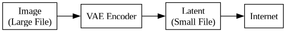
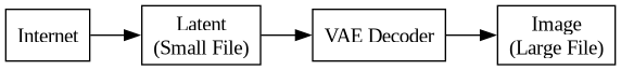
Assuming you already had the VAE decoder installed on your device, you would decode the latents before displaying the images. There may be some compression artifacts, but if the VAE is well-trained then they should not be noticable.
So, what's the point of having the VAE in the stable diffusion pipeline?
The VAE exists because it's too computationally expensive to work in the high-dimensional "pixel space" where images live. It's better (i.e. more efficient) to work in lower dimensions.
The VAE Encoder converts high-dimensional images into latents during training or Image-to-Image tasks. Other inputs (text, canny edge maps, positional encodings) are converted to the same latent space (but not via the VAE Encoder) so that the latents can be combined before (and during) the reverse diffusion process.
Working in latent space allows us to solve a less computationally expensive problem. Instead of generating a good image via reverse diffusion, we need only generate a good latent.
We convert good latents to good images by sending the latents through the VAE decoder.
Latent Diffusion Model

Input: Random noise latent (optionally combined with with non-random conditioning latents from text, canny edge maps, etc).
Output: A generated (denoised) latent, which can be sent through the VAE decoder to be converted to an image.
Summary: Given the explanations in the previous sections, we can now see that a latent diffusion model is simply a diffusion model that operates in latent space. The term "Latent Diffusion Model" does not imply a specific architecture: only that an iterative reverse diffusion process happens in a low-dimensional latent space.
U-Net
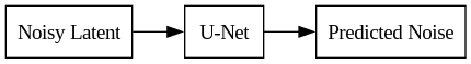
Input: Noisy image latents.
Output: Predictions of latent noise.
Terminology: When writing about Latent Diffusion Models, it's common to use the words "image", "latent", and "feature map" interchangably. This can be confusing, since the difference between pixel space and latent space is a critical innovation. However, the specific types of models that operate in latent space are usually not specifically limited to latents, images, or any particular type of input. So when discussing U-Nets, for example, the usual term to describe its inputs and outputs is "image", even though in our case, we'd think of them as "latents" or "latent images**.
Description: Stable Diffusion's U-Net is the central component in the reverse diffusion process. The U-Net is a specific network architecture whose structure enables it to efficiently process and understand spatial hierarchies within images. This makes it highly effective for tasks like image segmentation, denoising, and super-resolution.
In this case, Stable Diffusion's U-Net is fed latents and predicts which parts of its input are noise. A scheduler determines how to update the noisy input latent given the U-Net's prediction. This process continues iteratively until a predefined number of steps is reached. We call the final output of the U-Net the "denoised latent" and can convert it to an image via the VAE Decoder.
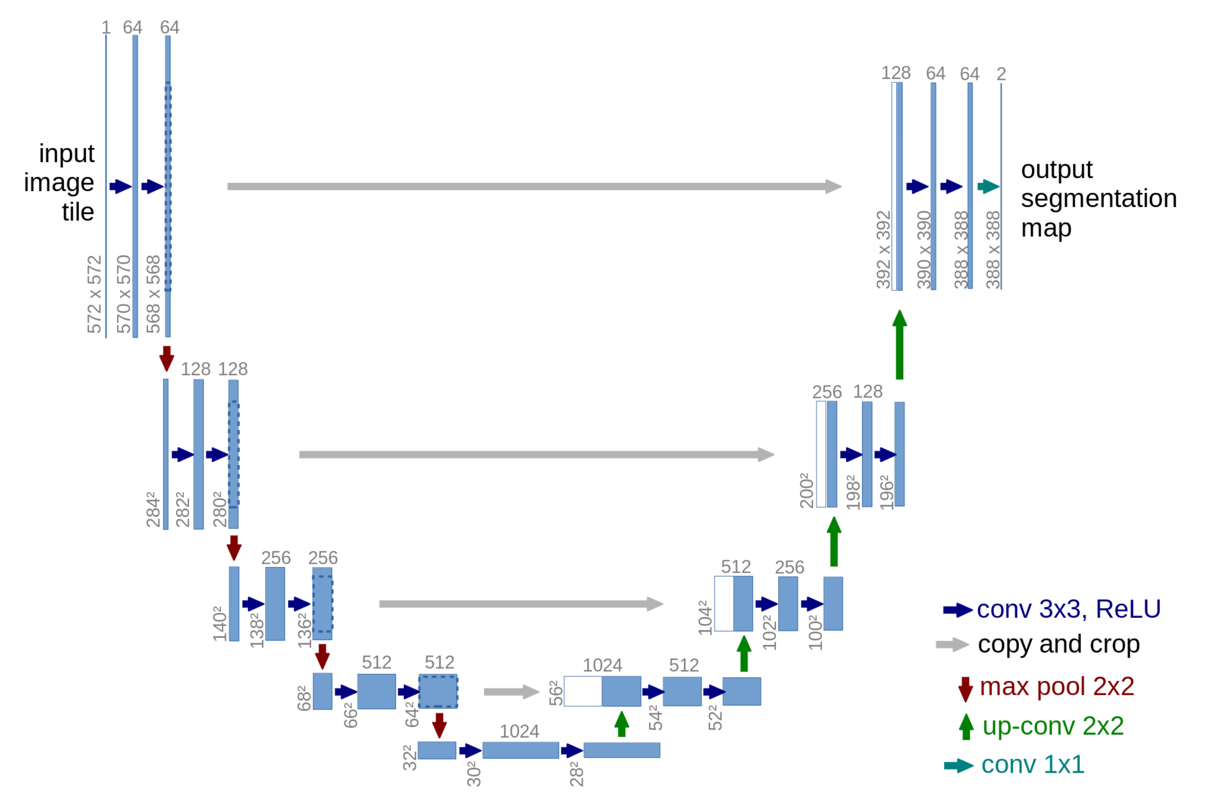
Clarification: Like an auto-encoder, a U-Net has a down-sampling "encoder", an up-sampling "decoder", and a low-dimensional "bottleneck" in-between. However, in general U-Nets and autoencoders are not the same. U-Nets are trained on a variety of tasks, whereas the term "autoencoder" refers to a two-sided networked trained to predict its own inputs. The terms "encoder" and "decoder** appear in several types of networks.
Key Concepts: A few key concepts explain why the U-Net is a good choice for image processing tasks.
- Convolution Layers: These layers apply a convolution operation to the input, capturing local dependencies and learning features from the data. In But what is a convolution, Grant Sanderson provides an excellent visual explanation of convolutions.
- Downsampling and Upsampling: Downsampling reduces the spatial dimensions (height and width) of the image, helping the model to abstract and learn higher-level features. Upsampling, conversely, increases the spatial dimensions, aiding in reconstructing the finer details of the image.
- Residual Connections: These connect layers of equal resolution in the downsampling and upsampling paths, allowing the model to preserve high-resolution features throughout the network. As with residual networks, these connections allow us to train deeper networked (networks with more layers) by alleviating the vanishing gradient problem.
CLIP (Contrastive Language-Image Pretraining)
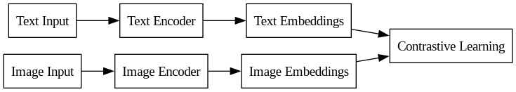
Input: Text and corresponding images.
Output: Text encoder and image encoder whose embeddings that are closely aligned in the embedding space.
Description: CLIP involves two encoders - one for text and one for images. The text encoder converts text inputs into embeddings, while the image encoder does the same for images. The core idea of CLIP is to train these encoders in a contrastive learning framework so that the embeddings of text and images that are semantically related are closer in the embedding space. In Stable Diffusion, we use a CLIP Text Encoder to convert text prompts to latents, and then condition our diffusion process on the text latents (by combining text latents with noise and other conditioning inputs).
Text Encoder
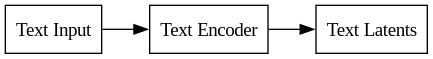
Input: Raw text data.
Output: Latent representations of the text.
Description: The Text Encoder (from CLIP) converts text prompts into a latents as described above. In Stable Diffusion, the text embeddings (latents) are used during the reverse diffusion process to condition the output. It's what allows us to do Text-to-Image tasks where the generated image is guided by a text prompt.
Control Net Conditioning Encoder

Input: Image conditioning data, such as Canny edge maps.
Output: Conditioning Latents.
Description: With Control Net, we want to condition the output of our diffusion process on canny edge maps, depth maps, segmentation maps or other types of data. But these data are not latents. For each control net (trained for a particular type of conditioning), we also create a small encoder network to transform our conditioning inputs into latent space, so that they can be properly combined with the other inputs.
Control Net Trainable Weights

Input: Conditioning Latents.
Output: Influences for the Stable Diffusion UNet.
Description: The central idea behind Control Nets is to create a trainable copy of Stable Diffusion's U-Net, connect the copy to the original via residual connections and "zero convolutions", and then train the copy with a dataset of conditional inputs/targets (while leaving the original U-Net weights alone). This idea is best explained by the recommended references, especially the original, well-written, very-readable research paper.
Alternative Methods of Fine-Tuning
Control Nets are not the only method of achieving a desired output. Nor are they exclusive. The following sections summarize a few additional ways to fine-tune a Stable Diffusion model.
Low-Rank Adaptation (LoRA)
Input: Original parameters of a pre-trained model.
Output: Adapted model parameters, with updates focused on specific aspects.
Description: Low-Rank Adaptation (LoRA) is a technique for fine-tuning pre-trained models in a parameter-efficient manner. Instead of updating all parameters, LoRA focuses on adapting a small subset, typically through low-rank matrices. This approach allows for efficient and targeted modifications of the model, often used to adapt large models to specific tasks or datasets without the computational cost of full model retraining.
Dreambooth

Input: A set of target images and a specified reference class.
Output: A generative model fine-tuned to generate images that include characteristics of the target images.
Description: Dreambooth is a technique used to fine-tune a pretrained generative model so that it can generate images containing specific characteristics of a given target. This is done by training the model with a set of target images, along with a reference class that the targets belong to. The result is a model capable of creating new images that maintain the essence of the target images, allowing for personalized or targeted image generation.
Textual Inversion

Input: A set of images depicting a specific concept and corresponding base text prompts.
Output: A language model adapted to understand and generate text related to the new, specific concept.
Description: Textual Inversion is a process where a pretrained language model is adapted to understand a new concept by training it with a set of images and associated text prompts. This method allows the model to incorporate a specific, often niche, concept into its understanding and generation capabilities. As a result, the model becomes more versatile in generating text that accurately reflects the new concept, enhancing its applicability to specialized or personalized tasks.
Glossary
It will help to collect definitions of several key terms, specifically in the context of their use in Stable Diffusion.
| Term | Definition |
|---|---|
| Autoencoder | A neural network with an encoder that compresses data into a latent space and a decoder that reconstructs the data from this compressed form. |
| CLIP | A method for training text encoders to produce embeddings that closely match associated image embeddings, used in various AI models for text-to-image tasks. |
| Conditioning | A process in diffusion models where external data (like text or edge maps) guides the generation of outputs, influencing the final image characteristics. |
| Control Net | An additional network in stable diffusion models for enhanced input conditioning, allowing for more specific control over the generated outputs. |
| Control Net Conditioning Encoder | Part of a control net, this component converts additional input data (e.g., edge maps) into a format compatible with the diffusion model's latent space. |
| Control Net Trainable Copy | A duplicate of the U-Net Encoder in Stable Diffusion that can be trained separately for added input conditioning, connected to the main encoder via zero convolutions. |
| Diffusion Model | A type of generative model that creates images by gradually reversing a process of adding noise to an image, ultimately revealing a coherent image. |
| Dreambooth | A training method used to personalize generative models, enabling them to produce content that reflects specific subjects or styles found in the training data. |
| Forward Diffusion | The process of incrementally adding noise to an image, progressively obscuring the original content, used in diffusion models. |
| Latent Diffusion Model | A diffusion model variant that operates in a compressed, low-dimensional latent space, offering improved performance compared to traditional high-dimensional models. |
| Latent Space | A compressed, lower-dimensional representation of data, used in models like autoencoders and diffusion models for efficient data processing. |
| Latents | Data representations in the latent space, typically compressed forms of higher-dimensional data like images or text. |
| Low-Rank Adaptation | A method for fine-tuning large models by altering only a small subset of their parameters, allowing for effective model improvements or adaptations with minimal changes. |
| Pixel Space | The high-dimensional space representing images, characterized by dimensions such as height, width, and number of color channels. |
| Reverse Diffusion | The step-by-step process of removing noise from an image in a diffusion model, gradually restoring it to a coherent form. |
| Stable Diffusion | A suite of latent diffusion models known for efficient and high-quality image generation, including versions like SD 1.4, SD 1.5, SDXL, and SDXL Turbo. |
| Text Encoder | A component that converts text into a latent representation, often used in conjunction with CLIP for text-to-image generation tasks. |
| Textual Inversion | A technique to adapt language models to understand and generate specific text or concepts not covered in their initial training, using targeted examples. |
| U-Net | A central model in Stable Diffusion, consisting of an encoder and decoder, that predicts the noise in image latents, adept at processing spatial hierarchies in images. |
| U-Net Decoder | The part of the U-Net that upscales and restores image details, using semantic information from the encoder to enhance image quality. |
| U-Net Encoder | The component of the U-Net that downscales images, capturing essential semantic information and preparing it for the decoding process. |
| VAE Decoder | The decoder part of a Variational Autoencoder, responsible for reconstructing images or data from compressed latent representations. |
| VAE Encoder | The encoder component of a Variational Autoencoder, which compresses input data into a latent representation. |
| Variational Autoencoder | A type of autoencoder that ensures random noise in the latent space can be decoded into plausible images, often used in generative tasks. |
Recommended References
These resources provide a deeper understanding of the concepts discussed. Of the many resources online, the author found these to be the most helpful and illuminating.
- Stable Diffusion: Explainer Video, fast.ai course lesson 9, fast.ai diffusion-nbs
- Control Nets: Research Paper, Paper Readthrough Video, Note on zero-convolutions
- Diffusion Models: Research Paper
- Latent Diffusion Models: Research Paper
- U-Net: Research Paper, Explainer Video
- Convolution: Grant Sanderson's video "But what is a convolution?"
- CLIP: Website, Research Paper
- Variational Auto-Encoders: Research Paper, Explainer Video
- ResNets: Explainer Video 1, Explainer Video 2
- Low-Rank Adaptations: Research Paper
- History of diffusion models: deepsense.ai blog post
